We now turn to spreadsheets, another major type of program used by computer users. We have already discussed word processors, which includes Microsoft Works Word Processor and Microsoft Word. Those programs enabled us to enter in words and data in the form of letters, reports, etc… In spreadsheets, we enter in either numbers, words/titles or formulas in order to have the computer perform mathematical calculations for us. Spreadsheets are nothing more than really quick, efficient and widely talented calculators. The spreadsheet which we will discuss is Microsoft Excel, however, this lesson is also applicable for Microsoft Works' spreadsheet.

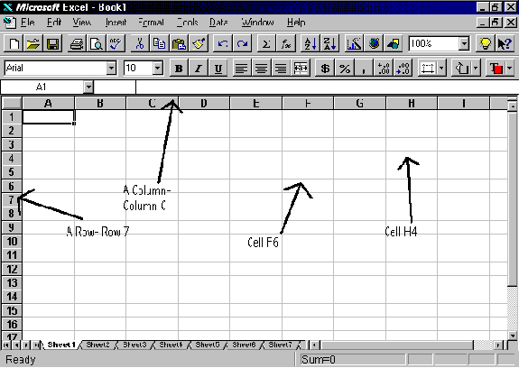
The screen of a spreadsheet is split into columns and rows. Each column and row come together at a specific location on the screen to form a cell. Each cell has a letter and number to identify it, which can be obtained from the letters on the horizontal top bar above the spreadsheet and the vertical numbers along the left side of the spreadsheet.

In cells we enter in the information. We can do calculations of the information which we enter, such as addition, multiplication, division, subtraction, average, logarithms, and many more complicated statistical calculations (standard deviation, sum of squares, variance, etc...). An empty cell has the value of 0.

To move around a spreadsheet, we use the arrow keys. We go to the cell we want to enter data into and then type in the data and press enter to have the data saved into that cell. If we don't press enter and use the arrow keys to go to another cell, then the data will be erased from that cell. We can edit the data in a cell by going to that cell using the arrow keys and then pressing delete to erase all the information in that cell and then reenter the information, or we can press F2 and then edit the information in that cell using a cursor which appears at the end of the cell, which you can move around and edit the data just like you did in a word processor.

Each cell has a width, which can be changed from the Format-Column-Width screen.

If you enter in data into a cell, and the data's width is larger than the column's width, then if you entered in numbers or the results of a formula, then the computer will display in that cell a bunch of characters as follows: ########, symbolizing that you should increase the column width. If you entered in a title or letters into the cell which are longer than the column width, then the letters will overlap into the next column, leading to a very poor display. The following examples show this:

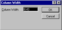
From the format-column-width menu, I choose to change the width of column A:

To

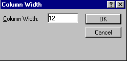
From the format-column-width menu, I choose to change the width of column B:

To

I then get the following results, which has column B being too small:

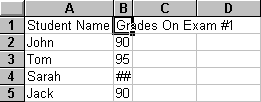
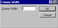
So I change the column width of column B to

We can enter in formulas to a cell. The format for entering in formulas is as follows:

When entering in a formula, always begin typing in the cell which will receive that formula an = sign. The equal sign tells the computer that you are entering in a formula. Next, say for example that you wish to add up the scores for exam #1 entered in the following spreadsheet:

You would type in cell #B6 the following: =b2+b3+b4+b5 and then press enter.

This is a valid formula which will add up the number values in cells b2, b3, b4 and b5 and then display the sum in cell b6 (note the capitalization of cell letters doesn't matter!). An easier way is to enter in the following formula: =sum(b2:b5). This formula tells the computer to perform a calculation, where it will take the sum of the values entered between cells b2 and b5 vertically down the column. The starting cell appears to the left of the colon and the ending cell to be included in the sum formula appears to the right of the colon.

I press Enter

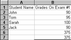
I can enter in some other formulas as well:

The formula MAX means to display the highest score between the range of cells given (from B2 to B5) and MIN is to display the lowest score between the given range (B2 to B5). Average takes the average of the scores from B2 to B5 {in Microsoft Works, you would type in =AVG(B2:B5) instead of =Average(B2:B5) }. With the results of these formulas, I get:

Instead of having to refer to another cell to perform a formula or calculation, I can just enter in the numbers I want to perform a calculation on in a formula with the appropriate mathematical or statistical function:

With the results I get

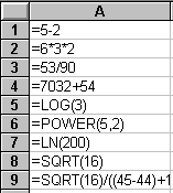
Note, SQRT is the square root function (or =SQR for Microsoft works) and POWER(5,2) raises 5 to the second power. LN in the natural logarithm and LOG is a logarithm.

I will now move on and create a new spreadsheet with more than one column as follows:

Say I want to find out the average on each exam, the highest and lowest scores on each exam and the average of each student. I would complete the following type of spreadsheet:

I enter in the formulas:

I get these results:

Now, say I want to get the average of each student. I could enter in the average formula in Column D for each student, or I could just enter in the formula once:

And then select using the F8 button and the down arrow key, the cells corresponding to where I want the average formula to appear for the other students:

And then choose Edit-Fill-Down option from the Edit menu, which will copy the formula from the cell that was first highlighted (D2) and copy the formula to the highlighted vertical cells (D3, D4 & D5). This saves a lot of time, especially if you have hundreds of students.

The computer then readjusts the formula to fit each row (from =AVERAGE(B2:C2) it changes to =AVERGAGE(B3:C3) and so on). You can also copy a formula across a row using Edit-Fill-Right or Left depending on which cell was highlighted first.

The results of this spreadsheet are as follows:

I can also edit the appearance of titles and data in a spreadsheet just like we did in Microsoft Word. You have to select which cell or cells are to be edited using the F8 key and then choose an editing option from the top of the screen.

Here, I chose to change the font size from 10 to 12:

I went out of my way to really fancy up this spreadsheet as can be seen in the following picture (can you tell what changes I made??):

You can also make charts and graphs in a spreadsheet. To do so, you must first select what data you want to graph using the F8 key as follows:

Next, choose to create a new chart from the tools-charts menu. You then get the following screen, where it displays the range of values that it will graph, which you have chosen (from A1 to A5 over to C1 to C5):

After clicking on Next, you get the following screen with a choice of graphs to choose from:

After choosing what type of graph you want and clicking on next, you get a sub-menu where you get to pick sub graph types. Here I chose #6:

You then get some additional options, which you generally need not change, so I clicked Next:

You then get the following screen, where you get to enter in a chart title, and titles for the X axis and the Y axis as shown:

After clicking on Finish, the completed chart appears in your spreadsheet and can be enlarged or shrunken using the black boxes on the edges of the chart just like we did in Microsoft Publisher. You can also move the chart around the screen.

We have now completed most of the common options of Microsoft Excel and spreadsheets in general. If you need any additional help, Microsoft Excel comes with a great help section, including an answer wizard, available from the help menu:

Goto --> Table of Contents